CORRELATING
VOLATILITY, VOLUME, CHANGE , AND TIME
BACKGROUND
One of the first questions that we posed in our project was is there any persistence between a stocks activity one day and its activity the following day. In order to answer this question we looked at the stocks volatility, volume, and daily change. The volatility of a stock is a measure of how much the stock moves in one day. This was measured this by taking magnitude of movement of the stock, (the daily high - the daily low) as a percentage of the original or opening value of the stock. We then performed experiments using all of the stocks on the DOW and looked over their entire history. The correlation coefficients were computed of a stocks properties one day with that from the day before, two days before, etc.. back until two months before. We computed the standard correlation coefficient which yields a number between –1.0 and 1.0. On the scale –1.0 is completely negatively correlated, 0 is no correlation, and 1.0 is complete correlation.
RESULTS
The Results we found were very interesting. An example of a typical stock that we looked at is MacDonald’s (MCD)
|
NUMBER DAYS BACK |
VOLATILITY CORRELATION |
STOCKS CHANGE CORRELATION |
|
1 |
0.441 |
0.021 |
|
2 |
0.371 |
-0.016 |
|
3 |
0.337 |
-0.024 |
|
4 |
0.311 |
-0.016 |
|
5 |
0.319 |
0.004 |
|
10 |
0.287 |
0.005 |
|
20 |
0.249 |
-0.012 |
|
30 |
0.264 |
-0.001 |
|
40 |
0.233 |
0.005 |
|
50 |
0.209 |
-0.002 |
There is a relatively high degree of correlation between a stocks volatility one day and a stocks volatility the next day over its history. However there is little to no correlation between the change one day and the following day. The average correlation between a stocks volatility one day and that of the previous day is about .46 for all of the stocks that we looked at. This is a significant amount. As the number of days back gets longer this number drops off quickly at first and then more slowly. There is still a fair amount of correlation even going back as far as two months. . Additionally there is a strong correlation between the volatility and the volume of a stock.
APPLICATIONS OF OUR RESULTS
We used this information to try and simulate the stock market. We knew that it would be very difficult to predict the absolute change of a stock based on its past history, but we could with some accuracy predict the volatility. Once we had a volatility prediction we could then use that volatility to try and predict what levels the stock was likely to hit in a given time period, as well as what price it was likely to close at over a given time period. We did this by running millions of random walk simulations of the stock that matched our predicted volatilities, and analyzing the results.
PREDICTING VOLATILITY
Now that we saw how the volatility changed with time we needed a model to help us predict the future volatility from the history of previous volatilities. Our results showed us that the volatility is very correlated with the previous days volatility, less so with the day before that, etc. We chose an “Exponentially Weighted Moving Average”(EWMA) to model this phenomenon and to predict the next day’s volatility. This model uses a coefficient to weight the contribution of the previous days contribution and then the day before gets weighted by this coefficient squared, and so on. Thus the predicted value will depend on a large amount of previous days values, but the most recent ones will be weighted the greatest. This is analogous to the results that we found in our experiment. The results produced by this predictor were fairly accurate and much better than simply using the previous days volatility as the predictor.
STOCK MARKET SIMULATION
RANDOM WALKS
Now that we had a good model for predicting the next days volatility we had to use this volatility to help forecast the stocks activity. We did this by setting up a simulation of the stock market and then running this simulation for volatility values that conformed to our predicted volatility. The simulation of the market that we choose is a random walk model. In this model the days trading is modeled as 1000 ticks or points in time. At each of these points in time the stock can either move up or down by some given step size. The probability of the stock moving up or down is completely random (a 50/50 chance). We then plot the value of the stocks movement and see the resulting volatility. This simulation is done millions of times for each step size, and then the volatility is averaged. I have created an applet which plots these simulations for a given volatility size, and number of days. This applet can be found at applet This gives us a mapping from a volatility value to a corresponding step size value. Once we know what step size the given volatility corresponds to we can then run a large amount of simulations of our random walk model with this step size to see maximum and minimum levels that the stock is likely to reach as well as what value the stock is likely to close at in a given amount of time. In order to not have to recalculate the same values over and over again we ran the simulation first to produce tables, of the percentage of time the stock reached and closed at certain levels and then we simply have to look at the appropriate table for a given volatility.
ACCURACY OF OUR MODEL
To test how accurate our methods were we went through the history of the stock and tested how we would have performed if we had used our predictor. For each day we predict the volatility of the next day using our EWMA model. Then we look at the maximum level that the stock reached the next day, the day after and so on. We consult our tables to see what we predicted the likelihood that the stock reached this level using our simulation. We did analogous analysis for the closing price of the stock. If our model was completely accurate we would expect to have an even distribution of the probability we predicted. We noticed quite quickly that as the number of days got larger into the future our model performed worse and worse. We realized that part of the reason for this is that our stock model simulation did not take into account how a stock moves in the time the market is closed. In reality a stocks closing price one day is not the same as it’s opening price the next day. The stock moves during the course of the night. We had to incorporate this movement into our simulation in order to make it more accurate. Thus we had to closely study the movement of stocks over the course of the night. Our results can be found at night.
Incorporating the night-moves of the stocks helped our results become more accurate. However, we saw that there was still room for improvement. We focused on our random walk model used in our simulation in order to make these improvements.
MODEL WITH HURST
Our original model resulted in a 50/50 chance of moving up/down at each step. This model has the desired property of producing no biased results (same chance of moving up or down). In reality the market has a slight upward bias, but this can be accounted for in our model by changing the probability of moving up/down from 50/50. This model was not completely ideal. It seemed unrealistic because it does not correctly seem to catch the momentum that the actual stock market exhibits. This means that market often gains momentum in one direction which makes movement in that direction more likely. For example consider extreme down days (crashes) in the market history. The market moved down to a much larger extent then would be expected just by 50/50 chance at each step. Rather there was a downward force that resulted in extreme movements. Every day there are forces acting on stocks or the market which produce some momentum. For example if a company reports better then expected earnings that stock will likely move up. This momentum is responsible for producing actual some stock movements that would be very rare with our random walk model.
RESULTS
In order to test how accurate our results were we produced tables of our model. These tables gave the likelihood that we moved up by a given gain and number of days. These tables were then mapped to their appropriate volatility. In order to test our results we looked at the last two years of market data. Each night we analyzed what the predicted volatility was for the next day. Mapped that volatility to the appropriate table. We then looked over the next 10 days and for each day noted the actual amount that the stock moved up(highest level it reached). We then found what percentage we predicted that that level would be hit in that amount of time according to our simulation. We added to the “bucket” representing that range of predicted percentages. For example if over 3 days the stock hit a high of 2% gain, and for that predicted volatility our simulation said there was a 25% chance that a stock would move up by 2% over 3 days, we would increase the bucket representing 30%-20% predicted. In this manner we analyzed how our predictions matched reality. Since our prediction is being run starting from the night before using the markets close the previous day as the starting point, there are times when the market will open the next day below the previous day close. In these cases its possible that over the next day the market never re-reaches the previous day close. Thus the high reached is negative. We ran our simulation in the same manner in order to predict this “negative bucket”. If our prediction is ideal this “<0%” should match reality. Then the other buckets should be all equal, divided among the remaining amount (those not in the “<0% bucket” ) Also, ideally there should be no days times that reach a high greater then our simulation predicted it ever would the “>100% bucket”. Here are our results:
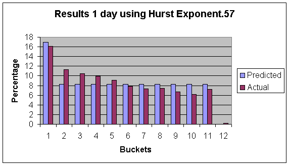
In this figure: Bucket 1 is “<0%” Bucket, 2-11 are divided among the remainding percentages equally, and Bucket 12 is “>100%”.
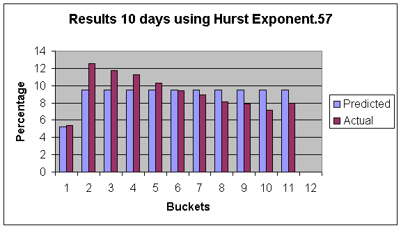
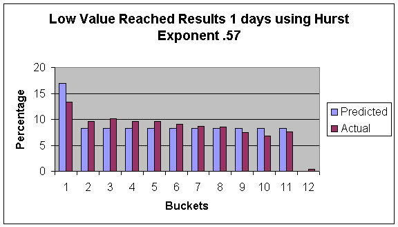
As can be seen by these figures, there is actually more times that the stock moves up by a small amount then we predict using our model. However the range of our prediction is quite accurate, (there is not a lot of days that go pass the maximum that our simulation predicted.) These results gradually get worse as the time in the future gets greater. The 10 day prediction is less accurate then the one day prediction. We focused on the previous two years to ignore problems that occurred before decimalization. It is noteworthy that the last two years have been a historically down time in the market, and therefore these results may be different in upward market. This can account for some of the highs reached not being as high as we predicted with our simulation. In order to see how much of an impact this phenomenon had I tested the data to predict losses. The experiment was identical only now I looked at the lowest point reached in an amount of time. Our prediction did better in this case, although this still followed the same trends of over-predicting the larger gains.
In addition to predicting the high values the price would reach we also tried to use our models to predict the closing value of the stock x days in the future. We evaluated our results in the same manner. Only here I used smaller buckets (every 4%) to see a finer picture of what was occurring. Here are the results:
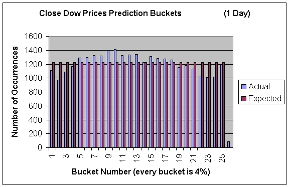
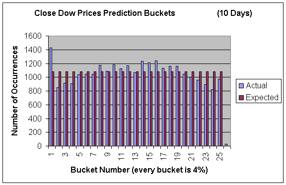
Our model predicted the closing prices reasonably well. Although there does tend to be more “mass” around the center suggesting that we are slightly over-predicting the bigger movements. Also, there tends to be more mass in the lower buckets but this can partially be explained by the market performance being poor since the start of decimalization.